Algorithms: An Introduction (Part 1)

13 Jan '24

This article introduces the basic algorithms that one would usually cover in a Data Structures and Algorithms course. It's not meant to be a comprehensive or technical piece, but rather to cover the big ideas on algorithms.I decided to write this article as a form of revision for the DSA book, Ace Your Next Coding Interview by Learning Algorithms through Programming and Problem Solving, which is written by Alexander Kulikov and Pavel Pevzner. The contents in the book are rephrased to demonstrate my understanding. It is supplemented with my prior knowledge, other books and websites. I hope that people who read this will find it useful as well. Ready? Let's begin... :)

What is an algorithm? An algorithm is a sequence of instructions that one must perform in order to solve a well-formulated problem (Kulikov & Pevzner). An algorithm is not confined to the domain of computer science. Think of cooking recipes and finding the highest common factor (greatest common divisor). One is in the domain of cooking and another is in mathematics, although one can solve the HCF by programming the algorithm in a computer.

Running Time of Algorithms

Given the choice between two or more algorithms that produce the same output barring any side-effects, computer scientists and programmers will want to implement the fastest algorithms as it saves time. Measuring the true running time of algorithms is not a scalable and feasible approach as it is affected by hardware factors like processor speeds, which is constantly improving. A better measure would be to calculate the algorithm's total number of operations. However, it is not easy to calculate the exact number of operations. A more feasible way would be to have a high-level understanding of the growth of the algorithm's operation count as the size of the input increases (Kulikov & Pevzner). What does it mean then? In studying the running time of algorithms, one is not interested in small values of input, n. What is of interest is the measure of growth of the algorithm as n becomes large.

Big-Oh Notation

The Big-Oh notation is a function which defines the limits of the growth of the algorithm. It is a measure of the algorithm's worse case efficiency. For example, if an algorithm has a Big-Oh represented by the function f(n) = O(n²), it would mean f(n) does not grow faster than a function with a leading term of cn². In Big-Oh notations, the coefficient and trailing terms are ignored. A more precise definition of the Big-Oh can be defined from the following. Consider two algorithms with running times of f(n) and g(n), where n is the input size. The function f grows no faster than g if there exists a constant c such that f(n) ≤ c.g(n), leading to the notation, f = O(g).

In the sections that follow, we will look at some common algorithm designs. Many algorithms are created based on these algorithmic designs.

A) Brute-Force Algorithms

Brute-Force Algorithms are also known as exhaustive search algorithms. In searching for an item, it would traverse an entire map or maze without any strategy. While it almost certainly ensures the item is found, it is inefficient. In designing algorithms, one should as much as possible avoid brute-force algorithms.

B) Branch and Bound Algorithms

Branch and bound is an algorithm design which is generally used for solving combinatorial optimisation problems. These problems are typically exponential in terms of time complexity and may require exploring all possible permutations in worst case. A famous example is The Travelling Salesman Problem (TSP). The problem statement is as such:

"Given a set of cities and the distances between each pair of cities, a salesman uses the shortest distance to visit each city exactly once and returns to the starting city."

There is no algorithm that can solve all instances of TSP optimally. The branch and bound algorithm works by systematically exploring the solution space, keeping track of promising candidates, and eliminating branches of the search space that cannot lead to an optimal solution. For TSP, it involves techniques and heuristics to efficiently explore the solution space. While it may not guarantee finding the optimal solution for large instances due to the Nondeterministic Polynomial (NP)-hard nature of the problem, branch and bound algorithms can significantly improve the efficiency of the search process. Click here for an interesting read on understanding NP problems.

C) Greedy Algorithms

Greedy algorithms are iterative optimisation algorithms that make locally optimal choices at each step with the hope of finding a global optimum. While this strategy often leads to correct solutions and works well for many problems, it does not guarantee an optimal solution in all cases. An example in which greedy algorithm paradigm is used is in scheduling problems.

i) Scheduling Problem

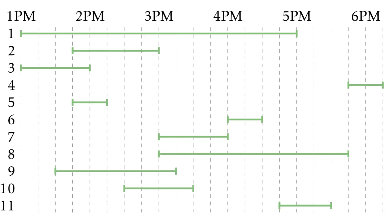
In the scheduling problem, the objective is to fit in as many bookings for a meeting room. A greedy approach could be to select the meeting with the shortest duration, remove meetings that overlap it, and iterate. This greedy approach algorithm seems sensible but it doesn't always work, as seen in the image below.

Let's try again then. Another sensible approach would be to select the meeting with the earliest start time, remove overlaps, and iterate. Again, it doesn't always work, as seen in the image below.

Having seen two greedy algorithms which may not work for all cases, is there a solution to it? The answer is yes. By selecting the right endpoint which is the smallest among all right endpoints, removing all intervals that overlap, and then iterating it, one would get the optimal solution to the scheduling problem.

ii) Haversack Greedy Algorithm

Let's look at another greedy algorithm problem. The Haversack Greedy Algorithm, also known as the Knapsack Greedy Algorithm, is an approach used to solve the knapsack problem, a classic optimisation problem in computer science. The problem is described as follows:

There is a set of items and a knapsack with a maximum weight capacity. Each item has a weight and value. The weight of an item could be represented by its actual weight or how much volume it occupies. The value can be thought of as a utility function like monetary value. The goal is to maximise the total value of items placed in the knapsack without exceeding its weight capacity.

The greedy algorithm works by iteratively selecting items to include in the knapsack based on a greedy criterion. The criterion involves selecting items with the highest value-to-weight ratio first, as this maximises the value gained per unit of weight.

Here's a step-by-step description of the Haversack Greedy Algorithm:

The Haversack Greedy Algorithm provides a relatively simple and efficient solution to the knapsack problem, particularly when the items are sorted based on their value-to-weight ratios. However, it's important to note that this algorithm does not always guarantee an optimal solution. For example, it may overlook certain combinations of items that could yield a higher total value than simply selecting items based solely on their individual value-to-weight ratios. The reason why a sub-optimal solution may be selected is due to the constraint set in the algorithm. Instead of exploring all possible solutions, the greedy constraint (e.g. highest value-to-weight ratio) restricts the search space for the optimal solution.

    Change(money, Denominations):
        numCoins <- 0
        while money > 0:
            maxCoin <- largest among Denominations that does not exceed money
            money <- money - maxCoin
            numCoins <- numCoins + 1
        return numCoins
    

The Change Greedy Algorithm displayed above is another example where the greedy algorithm produces a sub-optimal solution on using certain values e.g. Change(8,[1,4,6]). The algorithm above will result in 3 coins (6+1+1) when it can be achieved with a better result of 2 coins (4+4).

In conclusion while greedy algorithms offer a straightforward approach to solving optimisation problems and are often efficient, it's important to carefully analyse the problem to determine whether a greedy algorithm is appropriate and whether its solution is optimal.

D) Dynamic Programming Algorithms

Dynamic programming organises computations to avoid recomputing values that you already know, which can often save a great deal of time.

Dynamic programming is a method for solving complex problems by breaking them down into smaller, more manageable subproblems and solving each subproblem only once, thus saving time. The solutions to these subproblems are reused as needed. It is usually used in optimisation problems where the solution can be obtained by combining solutions to overlapping subproblems.

Let us analyse dynamic programming algorithms using the "Rocks" game. There are variations to this game and we will look into one of them; There are two piles of ten rocks each. In each turn, a player may remove either one rock (from either pile) or two rocks (one from each pile). The player who takes the last rock wins the game.

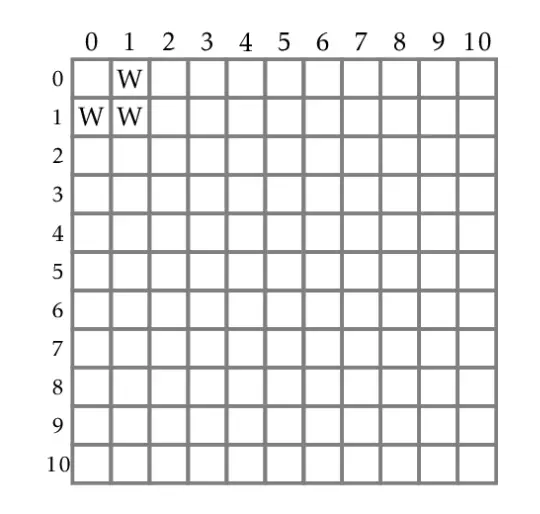
Let's visualise the pile of rocks using a 10 x 10 grid table, called R. The row and column each represents a pile. We can generalise the 10 x 10 table to a n x m table, implying n rocks in one pile and m rocks in the other. If, at the current state, Player 1 always wins the n + m game no matter what Player 2 does, then R(n,m) = W (Mark grid (n,m) with W). Likewise, R(n,m) = L if at the current state, Player 1 can never win against Player 2 (Mark grid (n,m) with L).

Having learnt how the cells should be filled up, we can start filling up the table. Cells (1,0), (1,1) and (0,1) would always result in Player 1 winning as Player 1 can make moves to remove all rocks based on the rules provided. We can fill up (2,0) next. As Player 1 can only remove 1 rock, it will result in (1,0), ensuring that Player 2 wins. Thus (2,0) is marked L. (0,2) is also marked L as it is just a matter of removing from the bottom pile instead of the top pile, all else being equal (symmetrical).

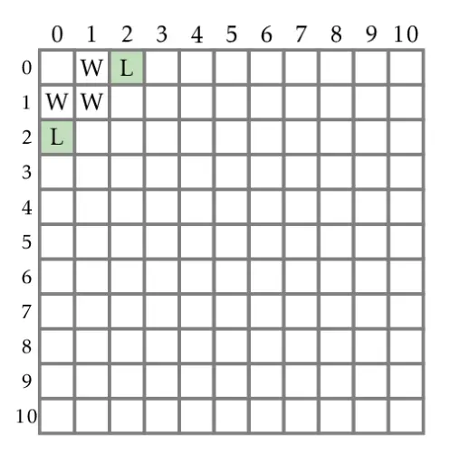
We have filled up 5 boxes so far. Let's proceed to fill up (2,1). Player 1 can make one of 3 moves, resulting in (2,0), (1,0) or (1,1). Assuming the game is played optimally (Player 1 removes 1 rock from the bottom pile resulting in (2,0)), (2,1) results in a winning move for Player 1 as Player 2 can only remove 1 out of 2 rocks from the bottom pile. Thus R(2,1) is marked W. As (1,2) is symmetrical to (2,1), R(1,2) is also marked W.

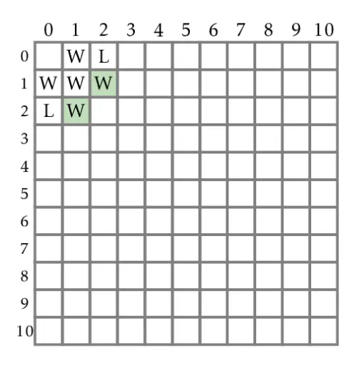
We use the same approach of determining the winner for the other cells. In the (2,2) case, Player 1 can make three different moves that lead to (2,1), (1,2) and (1,1). As we have already filled up the cells for these states with W, they would be winning states for the next Player, which is Player 2. Thus R(2,2) is marked L.

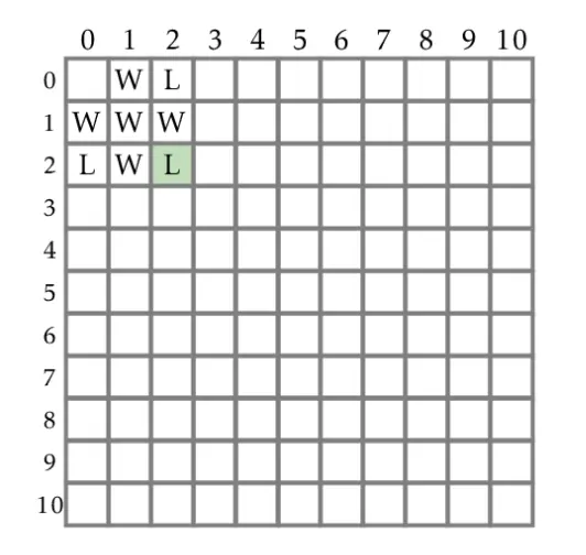
How can the table be filled up systematically (algorithmically) if there are n by m entries in the table? A commonly-used technique in problem-solving is to start with small values, scale it up, and notice if there is a pattern. If there is, it means there is an algorithmic approach to solving the problem. This is exactly what we have been doing. One can fill up the rest of table using the same reasoning.

In the Rocks game, a pattern can be established using this approach. We can quickly fill up the table by noticing that whenever a cell is marked L, the cells above, diagonally left and directly left are marked W. The completed table has the following entries below.

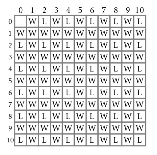
The Rocks game demonstrates dynamic programming where a complex problem is solved by broking it down into smaller subproblems. The solutions to the subproblems are used to solve the bigger problem and are used as needed.

We have gotten a taste of four approaches to designing algorithms, namely brute force, branch-and-bound, greedy algorithms and dynamic programming. Going through these algorithms, I realise that they were akin to solving puzzles. Those who enjoy puzzles will find a knack in this field. This concludes Part 1 of the Algorithms: An Introduction blog. In Part 2, we will explore Recursive Algorithms, Divide and Conquer Algorithms and Randomised Algorithms. Till next time. 😊